
1. What is a functional?
One says that a functional is given if a rule is fixed that associates a number to every function from certain function family. Thus, it is a mapping from a set of functions to a set of numbers. It is a generalization of the idea of a function of several variables to the realm of a function of infinitely many variables, the values of the argument function. For example, $sin(x^2)$ is not a functional. On the other hand
$$ \begin{equation} \tag{1.1} I_1[f]=\int_{0}^{1}f(x)dx \end{equation} $$
is a functional of $f$; it assigns a numerical value to the entire function, $f$. It is an analog of the finite sum $\sum f_i$.
Functionals can simultaneously be functions of a numerical variable. One example of how this can occur is
$$ \begin{equation} \tag{1.2} I_2[f;t]=\int_{0}^{1}g(x,t)f(x)dx \end{equation} $$
where $g$ is a given function of two variables. For fixed $t$ it is a functional of $f$ of the same type as $I_1$. Now let $f(x,t)$ be a function of two variables and consider
$$ \begin{equation} \tag{1.3} I_3[x,t]=\int_{0}^{1}g(x)f(x,t)dx \end{equation} $$
where $g$ is again some fixed function. This is another way that a functional can be an ordinary function at the same time. There are many other examples that could be invented of how this might occur.
Not all functionals are defined by integrals. The simplest example of one that is not is the Dirac delta ‘function, $\delta (x)$. This is often described as the function that is zero everywhere except at the origin, where it is infinite in such a way that
$$ \begin{equation} \tag{1.4} \int_{-\infty}^{\infty}\delta (x)dx=1. \end{equation} $$
Of course, there is no function for any reasonable definition of the integral sign. The delta ‘function’ is really a ‘functional’, assigning to any function, its value at origin. We may write
$$ \begin{equation} \tag{1.5} \delta [f]=f[0]. \end{equation} $$
This is what is really meant by the usual notation
$$ \begin{equation} \tag{1.6} \int_{-\infty}^{\infty}f(x)\delta (x)dx=f(0). \end{equation} $$
There is a differential and integral calculus for functions of finitely many variables. Is there an analog for ‘functionals’? Function spaces are huge and, in general it is not possible to define measures on them in a way that would mame integral calculus possible. But there are exceptional special cases. The Wiener integral is an integral of a functional over the space of continuous functions on an interval, albeit with a very special measure. The Feynman integral is also an integral of a functional over a function space. One the other hand, differentiation of functionals is possible. Suppose, we take a functional $I[f]$, and ask how it changes when we make a small change in $f$, to $f+\delta f$. This is the result of changes at all different values of $x$ in the domain of $f$ so we write it as
$$ \begin{equation} \tag{1.7} \delta I[f,df]=\int \frac{\delta I[f]}{\delta f(y)}\delta f(y)dy. \end{equation} $$
The quantity $\frac{\delta I[f]}{\delta f(y)}$ is called the functional derivative of $I$ with respect to $f$. It is the ceofficient of $\delta f$ in the linear part of the change in $I$. Equation (1.7) is analogous to the formula for the differential of a function of several variables $\delta f=\sum \left ( \partial f/\partial x_i \right )\delta x_i$. In general, the functional derivative $\frac{\delta I[f]}{\delta f(y)}$ is both a functional of $f$ and an ordinary function of $y$.
We now want to see how a functional changes as you adjust the function which is fed into it. Recall that a derivative of a function is defined as follows:
$$ \begin{equation} \tag{1.8} \frac{dI}{dx}=\displaystyle \lim_{\epsilon \to 0}\frac{I(x+\epsilon)-I(x)}{\epsilon} \end{equation} $$
The derivative of the function tells you how the number returned by the function $I(x)$ changes as you slightly change the number $x$ that you feed into the ‘machine’. In the same way, we can define a functional derivative of a functional $I[f]$ as follows
$$ \begin{equation} \tag{1.9} \frac{\delta I}{\delta f(x)}=\displaystyle \lim_{\epsilon \to 0}\frac{I[f(x’)+\epsilon \delta (x-x’)-I[f(x’)]}{\epsilon} \end{equation} $$
The functional derivative tells you how the number returned by the functional $I[f(x)]$ changes as you slightly change the function $f(x)$ that you feed into the machine.
Let $\delta f(y)$ be of the special form $\epsilon h(y)$ where $h$ differs from zero only in the interval $(y — \mu, y + \mu)$ and be such that $\int h(x)dx = 1$. Because the functional derivative is supposed not to depend on the increment $\delta f$, the integral on the right of eqn (1.7) may be approximated by
$$ \begin{equation} \tag{1.10} \delta I[f, \delta f(y)]=\epsilon \frac{\delta I}{\delta f(y)} \end{equation} $$
Thus
$$ \begin{equation} \tag{1.11} \frac{\delta I[f]}{\delta f(y)}=\displaystyle \lim_{{\epsilon \to 0},{\mu \to 0}}\frac{\delta I[f,\epsilon h]}{\epsilon} \end{equation} $$
Since $h(y)$ approximates the delta functional when used as an integral kernel, eqn (1.11) reduces to eqn (1.9).
Equation (1.9) leads to a formal expression that is often useful in evaluating functional derivatives expressed in the form of definite integrals
$$ \begin{equation} \tag{1.12} \frac{\delta f}{\delta f(y)}=\delta (x-x’) \end{equation} $$
2. Functional Representation of Problem Solution
Before really diving into this section, lets give some examples of functionals:
Here are some examples of functionals.
$(a)$. The functional $F [ f ]$ operates on the function $f$ as follows:
$$F [ f ] = \int _ { 0 } ^ { 1 } f ( x ) , d x .$$
Hence, given the function $f ( x ) = x^2$ , the functional returns the number
$$F [ f ] = \int _ { 0 } ^ { 1 } x ^ { 2 } , d x = \frac { 1 } { 3 } .$$
$(b)$. The functional G [ f ] operates on the function f as follows:
$$G [ f ] = \int _ { - a } ^ { a } 5 [ f ( x ) ] ^ { 2 } , \mathrm d x .$$ Hence, given the function $f ( x ) = x^2$ , the functional returns the number
$$G [ f ] = \int _ { - a } ^ { a } 5 x ^ { 4 } , d x = 2 a ^ { 5 } .$$
$(c)$. A function can be thought of as a trivial functional. For example, the functional $F_x[f]$ given by
$$F _ { x } [ f ] = \int _ { - \infty } ^ { \infty } f ( y ) \delta ( y - x ) \text {d} y = f ( x ).$$
returns the value of the function evaluated at $x$ .
$(d)$ $$ \quad F [ \varphi ( \tau ) ] = \overset { t _ { 2 } } { \int } d \tau a ( \tau ) \varphi ( \tau ) ,$$
where $a(t)$ is the given (fixed) function and limits $t_1$ and $t_2$ can be both finite and infinite. This is the linear functional.
$(e)$ $$\quad F [ \varphi ( \tau ) ] = \overset { t _ { 2 } } { \int } \overset { t _ { 2 } } { \int } d \tau _ { 1 } d \tau _ { 2 } B ( \tau _ { 1 } , \tau _ { 2 } ) \varphi ( \tau _ { 1 } ) \varphi ( \tau _ { 2 } ) ,$$
where $B(t_1,t_2)$ is the given (fixed) function. This is the quadratic functional.
$(f)$ $$F [ \varphi ( \tau ) ] = f \left ( \Phi [ \varphi ( \tau ) ] \right ) ,$$
where $f(x)$ is the given function and quantity $\Phi[\phi(\tau)]$ is the functional.
Variational (Functional) Derivatives
We now want to see how a functional changes as you adjust the function which is fed into it. The functional derivative tells you how the number returned by the functional $F [ f ( x )]$ changes as you slightly change the function $f ( x )$ that you feed into the machine.
Estimate the difference between the values of a functional calculated for functions $\phi(\tau)$ and $\phi(\tau)+\delta(\tau)$ for $t -\Delta \tau/2 < \tau < t + \Delta \tau/2$ (see Fig. 1.1).
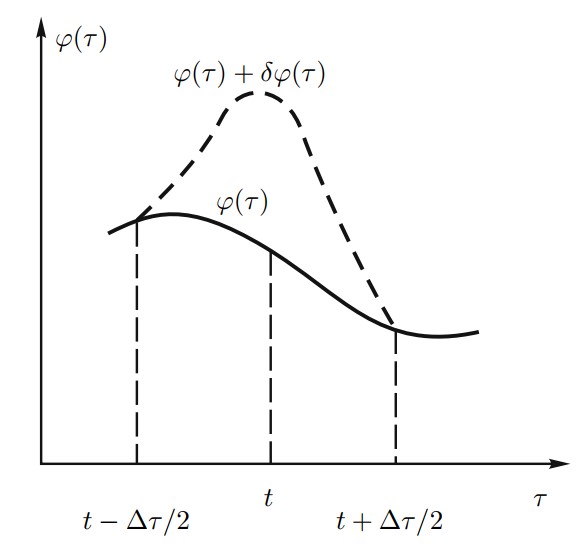
The variation of a functional is defined as the linear (in $\delta \phi (\tau)$ ) portion of the difference
$$\delta F [ \varphi ( \tau ) ] = { F \left [ \varphi ( \tau ) + \delta \varphi ( \tau ) \right ] - F [ \varphi ( \tau ) ] } , .$$
The limit $$ \begin{equation} \tag{2.1} \frac{}{}\frac{\delta F[\phi(\tau)]}{\delta \phi(\tau)dt}=\displaystyle \lim_{\Delta \tau \to 0}\frac{\delta \phi(\tau)}{\int_{\Delta \tau}^{}d\tau \delta \phi(\tau)} \end{equation} $$
is called the variational (or functional) derivative.
For short, we will use notation $\delta F [\phi(\tau)]/\delta \phi(t)$ instead of $\delta F [\phi(\tau)]/\delta \phi(t)dt$.
Note that, if we use function $\delta \phi(\tau) = \alpha \delta(\tau)$, where $\delta(\tau)$ is the Dirac delta function, then Eq. (2.1) can be represented in the form of the ordinary derivative
$$ \frac { \delta F [ \varphi ( \tau ) ] } { \delta \varphi ( t ) } = \lim _ { \alpha \to 0 } \frac { d } { d \alpha } F [ \varphi ( \tau ) + \alpha \delta ( \tau - t ) ]. $$
The variational derivative of functional $F[\phi(\tau)]$ is again the functional of $\phi (\tau)$, which depends additionally on point $t$ as a parameter. As a result, this variational derivative will have two types of derivatives; one can differentiate it in the ordinary sense with respect to parameter $t$ and in the functional sense with respect to $\phi (\tau)$ at point $\tau = {t}’$ thus obtaining the second variational derivative of the initial functional
$$\frac { \delta ^ { 2 } F [ \varphi ( \tau ) ] } { \delta \varphi ( t ^ { \prime } ) \delta \varphi ( t ) } = \frac { \delta } { \delta \varphi ( t ^ { \prime } ) } \left [ \frac { \delta F [ \varphi ( \tau ) ] } { \delta \varphi ( t ) } \right ] .$$
The second variational derivative will now be the functional of $\phi(\tau)$ dependent on two points $t$ and ${t}’$, and so forth.
Determine the variational derivatives of functionals ( a ), ( b ), and ( c ). In the case ( a ), we have
$$\delta F [ \varphi ( \tau ) ] = F [ \varphi ( \tau ) + \delta \varphi ( \tau ) ] - F [ \varphi ( \tau ) ] = \int _ { t - \frac { \Delta \tau } { 2 } } ^ { \Delta \tau } d \tau a ( \tau ) \delta \varphi ( \tau ) .$$
If function $a(t)$ is continuous on segment ∆τ , then, by the average theorem,
$$\delta F [ \varphi ( \tau ) ] = a ( t ^ { \prime } ) \int _ { \Delta \tau } d \tau \delta \varphi ( \tau ) ,$$
where point ${t}’$ belongs to segment $[t-\Delta \tau/2, t + \Delta \tau/2 ] $. Consequently,
$$\frac { \delta F [ \varphi ( \tau ) ] } { \delta \varphi ( t ) } = \lim _ { \Delta \tau \to 0 } a ( t ^ { \prime } ) = a ( t ) .$$
In the case ( b ), we obtain similarly
$$\frac { \delta F [ \varphi ( \tau ) ] } { \delta \varphi ( t ) } = \int _ { t _ { 1 } } ^ { t _ { 2 } } d \tau \left [ B ( \tau , t ) + B ( t , \tau ) \right ] \varphi ( \tau ) \ \left ( t _ { 1 } < t < t _ { 2 } \right ) .$$
Note that function $B(\tau_1, \tau_2)$ can always be assumed a symmetric function of its arguments here.
- First item
- Second item